Modelling parameter uncertainty and epidemic scenarios • epidemics

New to epidemics? It may help to read the “Get started” vignette first!

This vignette shows how epidemics can conveniently be used to:

Include parameter uncertainty in an epidemic model;
Run multiple scenarios of epidemic response measures;
Include parameter uncertainty when running multiple scenarios.

NOTE: This vignette applies only to the deterministic ODE models — the default, Vacamole, and diphtheria models. The Ebola virus disease model included in the package is expected to receive this functionality in the near future.

Code

# epi modelling
library(epidemics)
library(EpiEstim) # for Rt estimation

# data manipulation packages
library(dplyr)
library(tidyr)
library(purrr)
library(ggplot2)
library(colorspace)
library(ggdist)

# for reproducibility
library(withr)

Modelling parameter uncertainty

Uncertainty in the characteristics of an epidemic is a key element and roadblock in epidemic response (Shea et al. 2020). Epidemic dynamics can be influenced by two main sources of uncertainty: intrinsic randomness in the transmission process, and uncertain knowledge of the parameters underlying the transmission process. Here we focus on the latter, i.e. uncertainty in the input parameters of an epidemic model.

epidemics model functions can accept numeric vectors for all infection parameters; the model is run for each parameter combination using the same population and other model components (interventions, vaccinations) etc. This allows users to quickly obtain results for a range of parameter values without having to repeatedly call model_*() in a loop or similar; this iteration is performed internally.

Some benefits of vectorising inputs:

Inputs are checked all at once, rather than $N$ times for each element of the parameter vector — this improves performance over manual iteration;
Model output is organised to make filtering by parameter values and scenarios easier (more on this below).

Note that it is always possible to pass a single value of any infection parameter. Single values may be referred to as “scalar” values or “scalars”. Passing scalar infection parameters will yield a simple table of the model “time”, “demography group”, “compartment”, and “value”, for the number of individuals in each demographic group in each compartment at each model time point.

Click on “Code” below to see the hidden code used to set up a population in this vignette. For more details on how to define populations and initial model conditions please see the “Getting started with epidemic scenario modelling components” vignette. In brief, we model the U.K. population with three age groups, 0 – 19, 20 – 39, > 40, and social contacts stratified by age.

Code

# load contact and population data from socialmixr::polymod
polymod <- socialmixr::polymod
contact_data <- socialmixr::contact_matrix(
  polymod,
  countries = "United Kingdom",
  age.limits = c(0, 20, 40),
  symmetric = TRUE
)

# prepare contact matrix
contact_matrix <- t(contact_data$matrix)

# prepare the demography vector
demography_vector <- contact_data$demography$population
names(demography_vector) <- rownames(contact_matrix)

# initial conditions
initial_i <- 1e-6
initial_conditions <- c(
  S = 1 - initial_i, E = 0, I = initial_i, R = 0, V = 0
)

# build for all age groups
initial_conditions <- rbind(
  initial_conditions,
  initial_conditions,
  initial_conditions
)
# assign rownames for clarity
rownames(initial_conditions) <- rownames(contact_matrix)

Code

# UK population created from hidden code
uk_population <- population(
  name = "UK",
  contact_matrix = contact_matrix,
  demography_vector = demography_vector,
  initial_conditions = initial_conditions
)

Obtaining estimates of disease transmission rate

For this example, we consider influenza with pandemic potential (Ghani et al. 2010), and prepare multiple samples of the estimated $R$. This reflects pandemic response scenarios in which $R$ estimates always come with some uncertainty (due to limitations in the data and estimation methods). Sampling from a distribution that $R$ is expected to follow allows us to better understand the extent of variance in possible epidemic outcomes.

We obtain the probability distribution function (PDF) from the distribution of the serial intervals; this is a Gamma distribution with shape $k$ = 2.622 and scale $\theta$ = 0.957 (Ghani et al. 2010).

The forthcoming Epiverse package epiparameter is expected to make it substantially easier to access and use epidemiological parameters, such as the serial interval, reported in the literature, making it easier to model scenarios differing in the intrinsic characteristics of the pathogen causing the outbreak.

We use this PDF to estimate the $R$ of the 2009 influenza pandemic in the U.K., using the EpiEstim package. We use the $R$ estimate (the mean and standard deviation) from EpiEstim to generate 100 samples of $R$, assuming that it is normally distributed. Users who are drawing parameters with greater variance may wish to draw a larger number of samples.

Code

# Get 2009 influenza data for school in Pennsylvania
data(Flu2009)
flu_early_data <- filter(Flu2009$incidence, dates < "2009-05-10")

# get the PDF of the distribution of serial intervals
serial_pdf <- dgamma(seq(0, 25), shape = 2.622, scale = 0.957)
# ensure probabilities add up to 1 by normalising them by the sum
serial_pdf <- serial_pdf / sum(serial_pdf)

# Use EpiEstim to estimate R with uncertainty
# Uses Gamma distribution by default
output_R <- estimate_R(
  incid = flu_early_data,
  method = "non_parametric_si",
  config = make_config(list(si_distr = serial_pdf))
)

# Plot output to visualise
plot(output_R, "R")

Passing a vector of transmission rates

Here, we generate 100 samples of $R$, and convert to the transmission rate (often denoted $\beta$) by dividing by the infectious period of 7 days.

Since EpiEstim estimates $Rt$, the instantaneous $R$, we shall use the mean of the estimates over the time period, and the mean of the standard deviation, as parameters for a distribution from which to draw $R$ samples for the model.

Code

# get mean mean and sd over time
r_estimate_mean <- mean(output_R$R$`Mean(R)`)
r_estimate_sd <- mean(output_R$R$`Std(R)`)

# Generate 100 R samples
r_samples <- with_seed(
  seed = 1,
  rnorm(
    n = 100, mean = r_estimate_mean, sd = r_estimate_sd
  )
)

infectious_period <- 7
beta <- r_samples / infectious_period

Code

# pass the vector of transmissibilities to the argument `transmission_rate`
output <- model_default(
  population = uk_population,
  transmission_rate = beta,
  time_end = 600
)

# view the output
head(output)
#>    transmission_rate infectiousness_rate recovery_rate time_end param_set
#>                <num>               <num>         <num>    <num>     <int>
#> 1:         0.1977482                 0.5     0.1428571      600         1
#> 2:         0.2333557                 0.5     0.1428571      600         2
#> 3:         0.1885540                 0.5     0.1428571      600         3
#> 4:         0.2954036                 0.5     0.1428571      600         4
#> 5:         0.2397671                 0.5     0.1428571      600         5
#> 6:         0.1892204                 0.5     0.1428571      600         6
#>         population intervention vaccination time_dependence increment scenario
#>             <list>       <list>      <list>          <list>     <num>    <int>
#> 1: <population[4]>                                <list[1]>         1        1
#> 2: <population[4]>                                <list[1]>         1        1
#> 3: <population[4]>                                <list[1]>         1        1
#> 4: <population[4]>                                <list[1]>         1        1
#> 5: <population[4]>                                <list[1]>         1        1
#> 6: <population[4]>                                <list[1]>         1        1
#>                    data
#>                  <list>
#> 1: <data.table[9015x4]>
#> 2: <data.table[9015x4]>
#> 3: <data.table[9015x4]>
#> 4: <data.table[9015x4]>
#> 5: <data.table[9015x4]>
#> 6: <data.table[9015x4]>

The output is a nested <data.table>, with the output of each run of the model for each unique transmission_rate contained as a <data.frame> in the list column "data".

Output type for vector parameter inputs

The output of model_*() when an infection parameter is passed as a vector is a nested <data.table>. This is similar to a nested <tibble>, and can be handled by popular data science packages, such as from the Tidyverse.

More on handling nested data can be found in this section on list-columns in R for Data Science and in the documentation for nested data in the tidyr package. Equivalent operations are possible on <data.table>s directly; see this R Bloggers post on unnesting data.

We unnest the output’s “data” column in order to plot incidence curves for each transmission rate value.

Code

# select the parameter set and data columns with dplyr::select()
# add the R value for visualisation
# calculate new infections, and use tidyr to unnest the data column
data <- select(output, param_set, transmission_rate, data) %>%
  mutate(
    r_value = r_samples,
    new_infections = map(data, new_infections)
  ) %>%
  select(-data) %>%
  unnest(new_infections)

Code

# plot the data
filter(data) %>%
  ggplot() +
  geom_line(
    aes(time, new_infections, col = r_value, group = param_set),
    alpha = 0.3
  ) +
  # use qualitative scale to emphasize differences
  scale_colour_fermenter(
    palette = "Dark2",
    name = "R",
    breaks = c(0, 1, 1.5, 2.0, 3.0),
    limits = c(0, 3)
  ) +
  scale_y_continuous(
    name = "New infections",
    labels = scales::label_comma(scale = 1e-3, suffix = "K")
  ) +
  labs(
    x = "Time (days since start of epidemic)"
  ) +
  facet_grid(
    cols = vars(demography_group)
  ) +
  theme_bw() +
  theme(
    legend.position = "top",
    legend.key.height = unit(2, "mm")
  )

Incidence curves for the number of new infections on each day of the epidemic given uncertainty in the R estimate; colours indicate $R$ bins. Larger $R$ values lead to shorter epidemics with higher peaks, while lower R values lead to more spread out epidemics with lower peaks. Epidemics with $R$ < 1.0 do not 'take off' and are not clearly visible. Linking incidence curves to their $R$ values in a plot allows a quick visual assessment of the potential outcomes of an epidemic whose $R$ is uncertain.

Figure 1: Incidence curves for the number of new infections on each day of the epidemic given uncertainty in the R estimate; colours indicate $R$ bins. Larger $R$ values lead to shorter epidemics with higher peaks, while lower R values lead to more spread out epidemics with lower peaks. Epidemics with $R$ < 1.0 do not ‘take off’ and are not clearly visible. Linking incidence curves to their $R$ values in a plot allows a quick visual assessment of the potential outcomes of an epidemic whose $R$ is uncertain.

Passing parameter sets

epidemics model functions can accept multiple infection parameters as vectors, so long as any vectors are all of the same length, or of length 1 (scalar values) as shown below.

Code

beta <- rnorm(n = 100, mean, sd)
gamma <- rnorm(n = 100, mean, sd) # the recovery rate

model_default(
  population,
  transmission_rate = beta, # same length as gamma
  infectiousness_rate = 0.5, # length 1
  recovery_rate = gamma
)

Passing vectors of epidemic duration

epidemics allows the duration of an model run to be varied, as this may be useful when examining how variation in the start time of an epidemic affects outcomes by a fixed end point. This example shows how to estimate potential variation in the final epidemic size over a range of epidemic start times (and hence durations, assuming a fixed end).

Code

# draw samples of time_end
max_time <- 600
duration <- max_time - with_seed(seed = 1, {
  rnbinom(100, 1, 0.02)
})

Code

# view durations
ggplot() +
  geom_histogram(aes(duration)) +
  theme_bw() +
  labs(
    x = "Epidemic duration",
    y = "Count"
  )

Code

# pass the vector of durations to `time_end`
output <- model_default(
  population = uk_population,
  time_end = duration
)

# view the output
head(output)
#>    transmission_rate infectiousness_rate recovery_rate time_end param_set
#>                <num>               <num>         <num>    <num>     <int>
#> 1:         0.1857143                 0.5     0.1428571      589         1
#> 2:         0.1857143                 0.5     0.1428571      595         2
#> 3:         0.1857143                 0.5     0.1428571      568         3
#> 4:         0.1857143                 0.5     0.1428571      583         4
#> 5:         0.1857143                 0.5     0.1428571      589         5
#> 6:         0.1857143                 0.5     0.1428571      593         6
#>         population intervention vaccination time_dependence increment scenario
#>             <list>       <list>      <list>          <list>     <num>    <int>
#> 1: <population[4]>                                <list[1]>         1        1
#> 2: <population[4]>                                <list[1]>         1        1
#> 3: <population[4]>                                <list[1]>         1        1
#> 4: <population[4]>                                <list[1]>         1        1
#> 5: <population[4]>                                <list[1]>         1        1
#> 6: <population[4]>                                <list[1]>         1        1
#>                    data
#>                  <list>
#> 1: <data.table[8850x4]>
#> 2: <data.table[8940x4]>
#> 3: <data.table[8535x4]>
#> 4: <data.table[8760x4]>
#> 5: <data.table[8850x4]>
#> 6: <data.table[8910x4]>

NOTE: When the duration of the model runs is varied, each model output will have a potentially distinct number of rows.

Code

# calculate the epidemic size to view the mean and SD of sizes
epidemic_size_estimates <- select(output, param_set, data) %>%
  mutate(
    size = map(data, function(x) {
      tibble(
        demography_group = unique(x$demography_group),
        size = epidemic_size(x)
      )
    })
  ) %>%
  select(size) %>%
  unnest(size) %>%
  summarise(
    across(size, .fns = c(mean = mean, sd = sd)),
    .by = "demography_group"
  )

Code

# view the range of epidemic sizes
range(epidemic_size_estimates$size)
#> [1]  Inf -Inf

Modelling scenarios of epidemic response

Users may wish to model epidemic trajectories and outcomes under multiple scenarios of response measures.

epidemics model functions can accept lists of intervention sets and vaccination regimes, allowing multiple intervention, vaccination, and combined intervention-and-vaccination sets to be modelled on the same population.

Some benefits of passing lists of composable elements:

Combinations of intervention and vaccination scenarios can be conveniently created, as model functions will automatically create all possible combinations of the arguments to intervention and vaccination;
Input-checking and cross-checking is reduced by checking each element of the intervention and vaccination list independently before the combination is created (and against the population, for cross-checking); hence for $N$ intervention sets and $M$ vaccination regimes there are only $N+M$ cross-checks, rather than $N \time M$ cross-checks;
Model output is organised to provide a scenario identifier, making subsetting easier (more on this below).

It may help to read the “Modelling a non-pharmaceutical intervention targeting social contacts” and the “Modelling the effect of a vaccination campaign” vignettes first!

Which model components can be passed as lists

epidemics currently offers the ability to pass intervention sets and vaccination regimes as lists.

It is not currently possible to pass lists of populations, seasonality, or population changes to any models.

In future, it may be possible to pass multiple populations as a list, to rapidly and conveniently model an epidemic on different populations, or to examine the effect of assumptions about the population’s social contacts or demographic structure.

Creating a list of intervention sets

We shall create a list of ‘intervention sets’, each set representing a scenario of epidemic response measures.

Note that each intervention set is simply a list of <intervention> objects; typically, a single <contacts_intervention> and any <rate_interventions> on infection parameters.

Code

# prepare durations as starting at 25% of the way through an epidemic
# and ending halfway through
time_begin <- max_time / 4
time_end <- max_time / 2

# create three distinct contact interventions
# prepare an intervention that models school closures for 180 days
close_schools <- intervention(
  name = "School closure",
  type = "contacts",
  time_begin = time_begin,
  time_end = time_end,
  reduction = matrix(c(0.3, 0.01, 0.01))
)

# prepare an intervention which mostly affects adults 20 -- 65
close_workplaces <- intervention(
  name = "Workplace closure",
  type = "contacts",
  time_begin = time_begin,
  time_end = time_end,
  reduction = matrix(c(0.01, 0.3, 0.01))
)

# prepare a combined intervention
combined_intervention <- c(close_schools, close_workplaces)

Code

# create a mask-mandate rate intervention
# prepare an intervention that models mask mandates for 300 days
mask_mandate <- intervention(
  name = "mask mandate",
  type = "rate",
  time_begin = time_begin,
  time_end = time_end,
  reduction = 0.1
)

Having prepared the interventions, we create intervention sets, and pass them to a model function.

Code

# create intervention sets, which are combinations of contacts and rate
# interventions
intervention_scenarios <- list(
  baseline = NULL,
  scenario_01 = list(
    contacts = close_schools
  ),
  scenario_02 = list(
    contacts = close_workplaces
  ),
  scenario_03 = list(
    contacts = combined_intervention
  ),
  scenario_04 = list(
    transmission_rate = mask_mandate
  ),
  scenario_05 = list(
    contacts = close_schools,
    transmission_rate = mask_mandate
  ),
  scenario_06 = list(
    contacts = close_workplaces,
    transmission_rate = mask_mandate
  ),
  scenario_07 = list(
    contacts = combined_intervention,
    transmission_rate = mask_mandate
  )
)

Note that there is no parameter uncertainty included here. We can visualise the effect of each intervention set in the form of the epidemic’s final size, aggregating over age groups.

The output is a nested <data.table> as before — we can quickly get a table of the final epidemic sizes for each scenarios — this is a key initial indicator of the effectiveness of interventions.

Note that in this example, we use the model’s default $R$ estimate of 1.3. This is because at higher values of $R$, we get counter-intuitive results for the effects of interventions that reduce transmission. This is explored in more detail later in this vignette.

Code

# pass the list of intervention sets to the model function
output <- model_default(
  uk_population,
  intervention = intervention_scenarios,
  time_end = 600
)

# examine the output
head(output)
#>    transmission_rate infectiousness_rate recovery_rate time_end param_set
#>                <num>               <num>         <num>    <num>     <int>
#> 1:         0.1857143                 0.5     0.1428571      600         1
#> 2:         0.1857143                 0.5     0.1428571      600         1
#> 3:         0.1857143                 0.5     0.1428571      600         1
#> 4:         0.1857143                 0.5     0.1428571      600         1
#> 5:         0.1857143                 0.5     0.1428571      600         1
#> 6:         0.1857143                 0.5     0.1428571      600         1
#>         population intervention vaccination time_dependence increment scenario
#>             <list>       <list>      <list>          <list>     <num>    <int>
#> 1: <population[4]>                                <list[1]>         1        1
#> 2: <population[4]>    <list[1]>                   <list[1]>         1        2
#> 3: <population[4]>    <list[1]>                   <list[1]>         1        3
#> 4: <population[4]>    <list[1]>                   <list[1]>         1        4
#> 5: <population[4]>    <list[1]>                   <list[1]>         1        5
#> 6: <population[4]>    <list[2]>                   <list[1]>         1        6
#>                    data
#>                  <list>
#> 1: <data.table[9015x4]>
#> 2: <data.table[9015x4]>
#> 3: <data.table[9015x4]>
#> 4: <data.table[9015x4]>
#> 5: <data.table[9015x4]>
#> 6: <data.table[9015x4]>

Output type for list intervention inputs

The output of model_*() when either intervention or vaccination is passed a list, is a nested <data.table>. This is similar to the output type when parameters are passed as vectors, but with the "scenario" column indicating each intervention set as a distinct scenario, which helps with grouping the model outputs in "data".

The function epidemic_size() can be applied to the nested data column data to get the final size for each scenario.

Code

# set intervention labels
labels <- c(
  "No response", "Close schools", "Close workplaces", "Close both",
  "Mask mandate", "Masks + close schools", "Masks + close workplaces",
  "Masks + close both"
)

epidemic_size_estimates <- mutate(
  output,
  scenario = labels,
  size = scales::comma(
    map_dbl(data, epidemic_size, by_group = FALSE, include_deaths = FALSE)
  )
) %>%
  select(scenario, size)

# view the final epidemic sizes
epidemic_size_estimates
#>                    scenario       size
#>                      <char>     <char>
#> 1:              No response 23,084,960
#> 2:            Close schools 21,495,236
#> 3:         Close workplaces 22,423,830
#> 4:               Close both  6,622,568
#> 5:             Mask mandate 22,712,782
#> 6:    Masks + close schools 17,215,645
#> 7: Masks + close workplaces 20,564,673
#> 8:       Masks + close both  2,044,188

This example shows how implementing interventions that reduce transmission can reduce the final size of an epidemic.

Combinations of intervention and vaccination scenarios

When either or both intervention and vaccination are passed as lists (of intervention sets, or of vaccination regimes, respectively), the model is run for each combination of elements. Thus for $M$ intervention sets and $N$ vaccination regimes, the model runs $M \times N$ times, and each combination is treated as a unique scenario.

Note that ‘no intervention’ and ‘no vaccination’ scenarios are not automatically created, and must be passed explicitly as NULL in the respective lists.

While the number of intervention and vaccination combinations are not expected to be very many, the addition of parameter uncertainty for each scenario (next section) may rapidly multiply the number of times the model is run. Users are advised to be mindful of the number of scenario combinations they create.

The unnesting of the output follows the same procedure as before, and is not shown here.

Modelling epidemic response scenarios with parameter uncertainty

epidemics allows parameter uncertainty to be combined with scenario models of multiple intervention sets or vaccination campaigns.

Here, we shall draw 100 samples of the transmission rate with a mean of 0 and a low standard deviation of 0.005.

Code

beta <- with_seed(
  seed = 1,
  code = {
    rnorm(100, 1.3 / 7, 0.005)
  }
)

Code

# this example includes 100 samples of transmission rates for each intervention
# including the baseline
output <- model_default(
  uk_population,
  transmission_rate = beta,
  intervention = intervention_scenarios,
  time_end = 600
)

The output is a nested <data.table> as before, and can be handled in the same way.

Output type for intervention and parameter set combinations

The output of model_*() when either intervention or vaccination is passed a list, and when any of the infection parameters is passed as a vector is a nested <data.table>. The "scenario" column indicates each intervention set as a distinct scenario, while the "param_set" column indicates the parameter set used for the model run.

The same parameters are used for each scenario, allowing for comparability between scenarios at the aggregate level.

The output has $M \times N \times S$ rows (and nested model outputs), for $M$ intervention sets, $N$ vaccination regimes, and $S$ infection parameter sets.

Visualising parameter uncertainty in intervention scenarios

Here, we show one way of visualising the epidemic size across scenarios, accounting for parameter uncertainty.

Code

# select the data, the parameter set, and the scenario
epidemic_size_estimates <- select(output, param_set, scenario, data) %>%
  mutate(
    size = map_dbl(
      data, epidemic_size,
      by_group = FALSE, include_deaths = FALSE
    )
  ) %>%
  select(-data)

# Extract baseline and alternative scenarios
df_scenario1 <- epidemic_size_estimates %>% filter(scenario == 1)
df_scenarios_rest <- epidemic_size_estimates %>% filter(scenario != 1)

# Calculate differences as infections averted
df_differences <- df_scenarios_rest %>%
  left_join(df_scenario1, by = "param_set", suffix = c("_other", "_1")) %>%
  mutate(difference = size_1 - size_other) %>%
  select(param_set, scenario = scenario_other, difference)

Code

# Plot distribution of differences
ggplot(
  df_differences,
  aes(x = difference, y = factor(scenario), fill = factor(scenario))
) +
  stat_histinterval(
    normalize = "xy", breaks = 11,
    show.legend = FALSE
  ) +
  labs(
    title = "Scenario comparison",
    x = "Infections averted"
  ) +
  scale_x_continuous(
    labels = scales::comma
  ) +
  scale_y_discrete(
    name = NULL,
    labels = labels[-1]
  ) +
  scale_fill_discrete_qualitative(
    palette = "Dynamic"
  ) +
  theme_bw()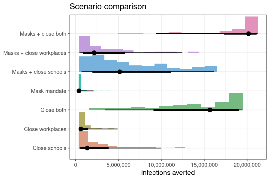

Infections averted relative to no epidemic response by implementing each scenario, while accounting with parameter uncertainty in the transmission rates.

Figure 2: Infections averted relative to no epidemic response by implementing each scenario, while accounting with parameter uncertainty in the transmission rates.

Counter-intuitive effects of time-limited interventions

The intervention scenarios modelled above suggest that:

interventions on disease transmission rates reduce infections and hence epidemic final sizes;
multiple interventions reduce epidemic final sizes more than single interventions.

In this simple example we show how this need not always be the case, and that counter-intuitively, implementing more interventions can lead to a larger epidemic final size than implementing fewer interventions.

This phenomenon depends on the baseline transmission rate of the infection, so we select a relatively low $R$ of 1.30 (corresponding to pandemic influenza), and a higher $R$ of 1.58 from the $R$ estimation step at the start of the vignette.

Code

# run each scenario for two values of R
# no parameter uncertainty
r_values <- c(1.3, round(r_estimate_mean, 2))

output <- model_default(
  uk_population,
  transmission_rate = r_values / 7,
  intervention = intervention_scenarios,
  time_end = 600
)

# obtain epidemic sizes
epidemic_size_estimates <- mutate(
  output,
  size = map_dbl(
    data, epidemic_size,
    by_group = FALSE, include_deaths = FALSE
  ),
  r_value = rep(r_values, each = length(intervention_scenarios)),
  scenario = rep(factor(labels, labels), 2)
) %>%
  select(r_value, scenario, size)

Code

# plot the epidemic final size for each scenario for each R
ggplot(epidemic_size_estimates) +
  geom_col(
    aes(scenario, size, fill = scenario),
    show.legend = FALSE
  ) +
  scale_x_discrete(
    name = NULL,
    guide = guide_axis(n.dodge = 2)
  ) +
  scale_y_continuous(
    labels = scales::comma,
    name = "Epidemic size"
  ) +
  scale_fill_discrete_qualitative(
    palette = "Dynamic"
  ) +
  facet_grid(
    cols = vars(r_value),
    labeller = labeller(
      r_value = function(x) sprintf("R = %s", x)
    )
  ) +
  theme_bw()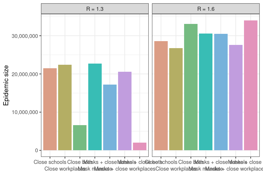

Counter-intuitive effects of time-limited interventions on transmission rate at high R values. Scenarios in which multiple interventions are implemented may have a larger final epidemic size than scenarios with fewer interventions, e.g. the 'Close both workplaces and schools' scenario.

Figure 3: Counter-intuitive effects of time-limited interventions on transmission rate at high R values. Scenarios in which multiple interventions are implemented may have a larger final epidemic size than scenarios with fewer interventions, e.g. the ‘Close both workplaces and schools’ scenario.

Plotting the epidemic trajectories for each scenario for each value of $R$ gives a fuller picture of why we see this unexpected effect.

Code

# get new infections per day
daily_incidence <- mutate(
  output,
  r_value = rep(r_values, each = length(intervention_scenarios)),
  scenario = rep(factor(labels, labels), 2),
  incidence_data = map(data, new_infections, by_group = FALSE)
) %>%
  select(scenario, r_value, incidence_data) %>%
  unnest(incidence_data)

Code

ggplot(daily_incidence) +
  annotate(
    geom = "rect",
    xmin = time_begin, xmax = time_end,
    ymin = -Inf, ymax = Inf,
    fill = "grey90", colour = "grey"
  ) +
  geom_line(
    aes(time, new_infections, col = as.factor(r_value)),
    show.legend = TRUE, linewidth = 1
  ) +
  scale_y_continuous(
    labels = scales::label_comma(scale = 1e-3, suffix = "K")
  ) +
  scale_colour_discrete_qualitative(
    palette = "Dynamic",
    name = "R"
  ) +
  facet_wrap(facets = vars(scenario), nrow = 2) +
  theme_bw() +
  theme(legend.position = "top") +
  labs(
    x = "Time since epidemic start",
    y = "New infections"
  )

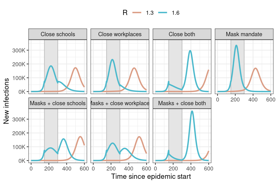
New daily infections in each intervention scenario for two values of R. The period in which interventions are active is shown by the area shaded in grey. No interventions are active in the 'No response' scenario.

Figure 4: New daily infections in each intervention scenario for two values of R. The period in which interventions are active is shown by the area shaded in grey. No interventions are active in the ‘No response’ scenario.

Implementing interventions on the disease transmission rate leads to a ‘flattening of the curve’ (reduced daily incidence in comparison with no response) while the interventions are active.

However, these cases are deferred rather than prevented entirely, and in both scenarios this is seen as a shifting of the incidence curve to the right (towards the end of the simulation period).

When $R$ is low, the incidence curve begins to rise later than when $R$ is high (interventions applied to these epidemics actually miss the projected peak of the epidemic, but still shift cases to the right). Thus low $R$ epidemics do not run their course by the time the simulation ends, making is appear as though interventions have succeeded in averting infections.

At higher $R$, the peak of the projected incidence curve without interventions falls within the intervention period, and thus all interventions reduce new infections. In scenarios with multiple active interventions, a large number of susceptibles remain uninfected, compared to scenarios with fewer interventions. The former thus see higher incidence peaks, leading to counter-intuitively larger final epidemic sizes.

Ghani, Azra, Marc Baguelin, Jamie Griffin, Stefan Flasche, Albert Jan Van Hoek, Simon Cauchemez, Christl Donnelly, et al. 2010. “The Early Transmission Dynamics of H1N1pdm Influenza in the United Kingdom.” PLoS Currents 1 (June): RRN1130. https://doi.org/10.1371/currents.RRN1130.

Shea, Katriona, Ottar N. Bjørnstad, Martin Krzywinski, and Naomi Altman. 2020. “Uncertainty and the Management of Epidemics.” Nature Methods 17 (9): 867–68. https://doi.org/10.1038/s41592-020-0943-4.