Getting started with modelling interventions targeting social contacts
Source:vignettes/modelling_interventions.Rmd
modelling_interventions.Rmd
library(epidemics)
library(dplyr)
#>
#> Attaching package: 'dplyr'
#> The following objects are masked from 'package:stats':
#>
#>     filter, lag
#> The following objects are masked from 'package:base':
#>
#>     intersect, setdiff, setequal, union
library(ggplot2)
Prepare population and initial conditions
Prepare population and contact data.
Note on social contacts data
epidemics expects social contacts matrices to represent contacts to from (Wallinga et al. 2006), such that is the probability of infection, where is a scaling factor dependent on infection transmissibility, and is the population proportion of group .
Social contacts matrices provided by the socialmixr package follow the opposite convention, where represents contacts from group to group .
Thus social contact matrices from socialmixr need to be
transposed (using t()) before they are used with
epidemics.
# load contact and population data from socialmixr::polymod
polymod <- socialmixr::polymod
contact_data <- socialmixr::contact_matrix(
  polymod,
  countries = "United Kingdom",
  age_limits = c(0, 20, 40),
  symmetric = TRUE,
  return_demography = TRUE
)
#> Warning: Automatic country population lookup in `contact_matrix()` was deprecated in
#> socialmixr 0.6.0.
#> When `countries` is given (or a `country` column is present) without
#> `survey_pop`, contact_matrix() currently calls the soft-deprecated `wpp_age()`
#> to look up population data. This automatic lookup will be removed in a future
#> release: callers will then have to supply `survey_pop` whenever `symmetric`,
#> `split`, `per_capita`, `weigh_age`, or `return_demography` is TRUE.
#> ℹ Pass `survey_pop` explicitly to silence this warning, e.g. `survey_pop =
#>   survey_country_population(survey, countries)` or a data frame from the
#>   wpp2024 package.
#> This warning is displayed once per session.
#> Call `lifecycle::last_lifecycle_warnings()` to see where this warning was
#> generated.

# prepare contact matrix
contact_matrix <- t(contact_data$matrix)

# prepare the demography vector
demography_vector <- contact_data$demography$population
names(demography_vector) <- rownames(contact_matrix)
Prepare initial conditions for each age group.
# initial conditions
initial_i <- 1e-6
initial_conditions <- c(
  S = 1 - initial_i, E = 0, I = initial_i, R = 0, V = 0
)

# build for all age groups
initial_conditions <- rbind(
  initial_conditions,
  initial_conditions,
  initial_conditions
)

# assign rownames for clarity
rownames(initial_conditions) <- rownames(contact_matrix)
Prepare a population as a population class object.
uk_population <- population(
  name = "UK",
  contact_matrix = contact_matrix,
  demography_vector = demography_vector,
  initial_conditions = initial_conditions
)
Prepare an intervention
Prepare an intervention to simulate school closures.
# prepare an intervention with a differential effect on age groups
close_schools <- intervention(
  name = "School closure",
  type = "contacts",
  time_begin = 200,
  time_end = 300,
  reduction = matrix(c(0.5, 0.001, 0.001))
)

# examine the intervention object
close_schools
#> <contacts_intervention> object
#>
#>  Intervention name:
#> "School closure"
#>
#>  Begins at:
#> [1] 200
#>
#>  Ends at:
#> [1] 300
#>
#>  Reduction:
#>              Interv. 1
#> Demo. grp. 1     0.500
#> Demo. grp. 2     0.001
#> Demo. grp. 3     0.001
Run epidemic model
# run an epidemic model using `epidemic`
output <- model_default(
  population = uk_population,
  intervention = list(contacts = close_schools),
  time_end = 600, increment = 1.0
)
Prepare data and visualise infections
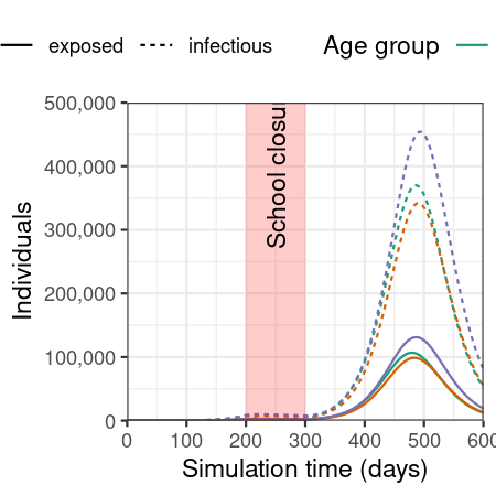
Plot epidemic over time, showing only the number of individuals in the exposed and infected compartments.
# plot figure of epidemic curve
filter(output, compartment %in% c("exposed", "infectious")) |>
  ggplot(
    aes(
      x = time,
      y = value,
      col = demography_group,
      linetype = compartment
    )
  ) +
  geom_line() +
  annotate(
    geom = "rect",
    xmin = close_schools$time_begin,
    xmax = close_schools$time_end,
    ymin = 0, ymax = 500e3,
    fill = alpha("red", alpha = 0.2),
    lty = "dashed"
  ) +
  annotate(
    geom = "text",
    x = mean(c(close_schools$time_begin, close_schools$time_end)),
    y = 400e3,
    angle = 90,
    label = "School closure"
  ) +
  scale_y_continuous(
    labels = scales::comma
  ) +
  scale_colour_brewer(
    palette = "Dark2",
    name = "Age group"
  ) +
  expand_limits(
    y = c(0, 500e3)
  ) +
  coord_cartesian(
    expand = FALSE
  ) +
  theme_bw() +
  theme(
    legend.position = "top"
  ) +
  labs(
    x = "Simulation time (days)",
    linetype = "Compartment",
    y = "Individuals"
  )